Session 02: Installing R packages, I/O + a deep dive into the data.frame class

2.1 Install a package to read data from Excel

What if the listings data frame was stored as a Microsoft Excel file, with an .xlsx extension in place of .csv? Well, one thing to do would be to first convert it to csv outside R, from Excel itself for example. Why would we do that? Because we tend to be consistent in the way we code and what procedures and standards do we use in our work: for example, we can introduce a convention to keep all data as .csv files in the scope of some project. But sometimes we don’t and we simply need to grab a file with a certain extension quickly. Now, base R does not have a function to read .xlsx files. But there are R packages that provide such functions. Whenever we want to use an R package, we need to install it first. The base R function to install packages is install.packages():

install.packages('readxl')

When we want to use functions from an R package, we need to call the package by library():

library(readxl)

Now, the readxl package has a function to read Excel files:

listings <- read_excel(paste0(dataDir, "listings.xlsx"), 
                       col_names = TRUE)
head(listings)

Note how I have reused the variable name: listings. It was an existing data frame which is now overwritten by the same data from a different file. Do not forget to use ? from the R console to obtain documentation on any new functions that you need to learn: ?read_excel, for example.

Note. Do class(listings):

class(listings)

What is this: tbl_df, tbl? In short: the classes were added to the data.frame class in the read_excel() call and we will start meeting them frequently once we begin to use the tidyverse packages like readr. Nothing to worry about at this point. Let’s strip them of the listings object manually:

listings <- as.data.frame(listings)
class(listings)

Ok. Back to the original listings.csv now:

filename <- paste0(dataDir, 'listings.csv')
listings <- read.csv(file = filename, 
                    header = T, 
                    check.names = F,
                    stringsAsFactors = F)

2.2 Subsetting a data frame in base R

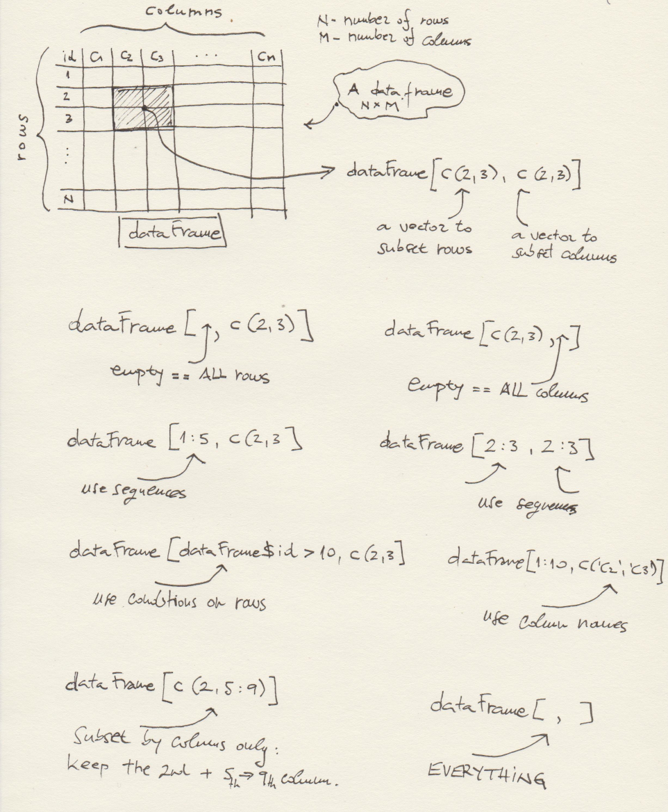
Now we need to learn how to subset a data frame, to slice out exactly the data that we are interested in. Data frames can be sliced by conditions set on their rows, columns, and by any combinations of conditions set on rows and columns. For example, if we are interested in only the top five rows of listings, we can do:

listings_5 <- listings[1:5, ]
listings_5

Remember head() - we can use that too:

listings_5 <- head(listings, 5)
listings_5

Again, the columns of listings:

colnames(listings)

And if we want to subset only the rows from 5 to 10 and only the name and room_type columns:

listings[5:10, c('host_name', 'room_type')]

Or:

listings[5:10, c(4, 9)]

Or:

listings[c(5,6,7,8,9,10), c(4, 9)]

Remember that c() puts things together in R. We have used two vectors, c(5,6,7,8,9,10), which can also be written as a sequence 5:10, and c(4,9) in which we have used column positions but we could have used column names as well like in the c('host_name', 'room_type') example to subset the listings data frame.

We can subset a data frame by imposing conditions on rows and/or columns too:

listings[listings$id > 42000 , c(2, 3)]

Shall we set a condition on column names perhaps?

2.3 Subsetting by columns + grepl() to perform regex match

listings[1:10, grepl("^number", colnames(listings))]

We already now that colnames(listings) will return a character vector encompassing all column names from listings. The grepl() function operates on characters. It’s task is to check if the regular expression (regex) described by its first argument (^number in our example) matches any character sequence found in its second argument (colnames(listings) in our example). The regular expression ^number says search for anything that begins with number in the given string, so ^ is the character (precisely: a metacharacter) in the regex syntax that stands for the beginning of the string. Similarly, $ is a metacharacter that stands for the empty character at the end of the string. Let’se see what grepl() does:

string <- 'the quick brown fox jumps over the lazy dog'
grepl('^t', string)

^^ Asks if string begins with 'T'.

string <- 'the quick brown fox jumps over the lazy dog'
grepl('g$', string)

^^ Asks if string ends with 'g'.

string <- 'the quick brown fox jumps over the lazy dog'
grepl('x$', string)

^^ Asks if string ends with 'x'.

strings <- c('the quick brown fox jumps over the lazy dog', 
             'Inland Empire', 
             'Wild at Heart')
grepl('e$', strings)

We will learn more about regex later in this course. But the previous example illustrates something more than the usage of grepl() to check for character sequences in R. Pay attention, please: we have defined a new character vector, strings, with three elements: 'the quick brown fox jumps over the lazy dog', 'Inland Empire', and 'Wild at Heart'. We have called grepl() like this: grepl('e$', strings) to ask if any of the strings in strings matches the e$ regex (and e$ asks: does it end with 'e'?). R responded by a vector of logicals: FALSE TRUE FALSE, and the length of the output vector is 3 - exactly as the length of the input string strings. In other words, grepl() is a vectorized function: it can be applied to a vector of elements, and will compute what it does on each element, pack its results back in another vector and serve them in that form! Many R functions are vectorized, and this is one the most powerful features of this beautiful programming language. We will also learn much more about vector programming and code vectorization with R in our future sessions.

A glimpse of vectorization only, the essential feature of R - which is a member of the class of vector languages or vector programming languages:

someVector <- c(1, 2, 3, 4, 5)
someVector + 10

someVector^2

someVector %% 2 == 0

2.4 read.csv() from the Internet

Oh, one more thing. Remember that listings live on the Internet: here. If you browse to that Inside Airbnb page and copy (right click!) the listings.csv link location - http://data.insideairbnb.com/the-netherlands/north-holland/amsterdam/2020-12-12/visualisations/listings.csv in the time of writing of this Notebook - you can obtain it from read.csv() in R like this:

urlData <- 'https://data.insideairbnb.com/the-netherlands/north-holland/amsterdam/2024-09-05/visualisations/listings.csv'
listingsOnline <- read.csv(URLencode(urlData), 
                           header = T, 
                           check.names = F, 
                           stringsAsFactors = F)
head(listingsOnline)

The URLencode() function takes care of the percent-encoding of characters in the URLs. Never forget to use it when you need an online file. There are better solutions to this than the base R URLencode() function (see: urltools package), but the base solution will do nicely as well - or at least in the beginning of your work in Data Science.

Now we have a copy of listings…

rm(listingsOnline)

Only our second session and we can already read data from the local filesystem, Microsoft Excel, and the Internet!

2.5 Subsetting data frames in base R: some principles

Ok, back to data.frame. Here are some principles of data frame subsetting in R:

3.1 Play for real: a deep dive into listings!

Ok. First, I would like to learn more about the calculated_host_listings_count column, which I did not understand immediately. I have an intuition about it: it could be the number of different listings with the same host_id/host_name.

Step 0: reload listings.csv

filename <- paste0(dataDir, 'listings.csv')
listings <- read.csv(file = filename, 
                    header = T, 
                    check.names = F,
                    stringsAsFactors = F)
str(listings)

Step 1: ask R how many unique host_id values there are in the dataset:

num_hosts <- length(unique(listings$host_id))
num_hosts

The unique() function: you will be using it every now and then. It’s easy: if vec <- c(1, 2, 3, 5, 5, 7) is a vector, unique(vec) is c(1, 2, 3, 5, 7), look:

vec <- c(1, 2, 3, 5, 5, 7)
unique(vec)

Step 2: ask R to count how many different listings there are per unique host_id.

num_host_listings <- table(listings$host_id)
head(num_host_listings, 50)

The table() function is your tool to obtain the frequency distribution of a variable in R. It’s easy: if vec <- c(1, 2, 3, 5, 5, 7, 7, 7) is a vector, table(vec) is:

vec <- c(1, 2, 3, 5, 5, 7, 7, 7)
table(vec)

What is the class() of the output of table()?

class(table(vec))

Yes, R has a plenty of specific types, and sometimes - and maybe most of the time - it is handy to turn them all into data frames:

freqHosts <- as.data.frame(table(listings$host_id), 
                           stringsAsFactors = FALSE)
head(freqHosts)

The Var1 represents the host_id from the listings data frame, while Freq is its frequency: how many times does the respective value of Var1 appear in the listings data.frame?

One check:

dim(freqHosts)[1] == num_hosts

Of course, it has to be! So dim(x) where x is a data.frame returns a vector of length two, of which the first element is the number of rows in x and the second the number of columns in x. In a frequency distribution, every particular value of a discrete variables occurs only once, so of course that dim(freqHosts)[1] == num_hosts must evaluate to T.

Now, if my intuition that calculated_host_listings_count column stands for the number of different listings with the same host_id/host_name, then its values must be the same as those that I have produced by table() in freqHosts. How do we test this hypothesis?

Step 3. Extract only host_id and calculated_host_listings_count from listings; if I am right, there will be duplicated values in this selection:

testHosts <- listings[ , c('host_id', 'calculated_host_listings_count')]
head(testHosts)

Ok, now: are there any duplicated rows present?

d <- duplicated(testHosts)
table(d)

Of course there are, but the result most probably does not mean too much at this point. Step by step, the duplicated() function R returns a logical vector (TRUE or FALSE):

vec <- c(1, 2, 3, 2, 2, 4, 5, 5, 7)
duplicated(vec)

Note how each first appearance of an element in a vector receives FALSE - because it is not duplicated - while every subsequent appearance of the same element receives TRUE - because it is duplicated. duplicated() works for data frames too, in which case it looks at all the values across all of the rows and returns as many logicals as there are rows following the same logic: first apperance is marked as FALSE and then all repetitions are marked as TRUE:

d <- duplicated(testHosts)
head(d)

So, what happened when I did table(d) is that R has counted how many duplicates (TRUE) there were in testHosts:

table(d)

There are 2489 duplicated values. Interesting enough, I can use the logical vector that duplicated() outputs to clean up my testHosts data frame from duplicated entries in this way:

dim(testHosts)

testHosts <- testHosts[!duplicated(testHosts), ]

dim(testHosts)

to keep only the 16033 rows that were never repeated.

We get back to the hypothesis: calculated_host_listings_count column stands for the number of different listings with the same host_id/host_name. If this is true, than the frequency counts in freqHosts$Freq must be the same, across the host_id values, as the values found in testHosts$calculated_host_listings_count, correct? How do we proceed to find out?

What do we have are two data frames:

head(freqHosts)

and the de-duplicated testHosts:

head(testHosts)

and do not forget that we know that Var1 in freqHosts encompasses the same values of host_id from listings as testHosts$host_id. I would know like to put freqHosts and testHosts side by side and inspect if the values of freqHosts$Var1 and testHosts$host_id are really the same.

Check one thing first:

dim(freqHosts)
dim(testHosts)

Of course. But the order of Var1 in freqHosts and host_id in testHosts does not seem to be the same. Let’s fix that by using order(). How does it work?

someDataFrame <- data.frame(someNum = c(5, 9, 1, 3, 4, 10), 
                            someChar = c ('a', 'b', 'c', 'd', 'e', 'f'), 
                            stringsAsFactors = F)
print(someDataFrame)

Now:

someDataFrame[order(someDataFrame$someNum), ]

Take a look at the following:

vec <- c(5, 9, 1, 3, 4, 10)
order(vec)

or

vec <- c(5, 9, 1, 3, 4, 10)
vec[order(vec)]

So, the output of order() tells us the following: which element of a vector (by position) should be placed where in order to have the original vector sorted out. This is why

someDataFrame[order(someDataFrame$someNum), ]

works: order(someDataFrame$someNum) returns an ordering of rows such that the data frame is sorted by someNum.

We now sort freqHosts and testHosts so that all host_id values are aligned (remember, Var1 in freqHosts represents hosts_id in testHosts). Before we do that, take a look at the following:

str(freqHosts)
str(testHosts)

What I do not like is that Var1in freqHosts is a character, while host_id in testHosts is a numeric. Fix:

freqHosts$Var1 <- as.numeric(freqHosts$Var1)
str(freqHosts)

Ok, sort freqHosts by Var1:

freqHosts <- freqHosts[order(freqHosts$Var1), ]
head(freqHosts, 10)

and sort testHosts by host_id:

testHosts <- testHosts[order(testHosts$host_id), ]
head(testHosts, 10)

Now the two data frames should be nicely aligned. Let’s put them side by side in a new data frame:

testDataFrame <- cbind(freqHosts, testHosts)
head(testDataFrame, 40)

Are the two data frames perfectly aligned? To find out we ask how many matches there are between testDataFrame$Var1 and testDataFrame$host_id:

sum(testDataFrame$Var1 == testDataFrame$host_id)

A new R function: sum(). This is how it works:

sum(c(5, 6))

But also:

sum(c(TRUE, FALSE, TRUE, TRUE))

sum() across logical vectors in R: TRUE counts as 1, FALSE counts as 0. So if we derive an index vector, say something indicating the number of matches of some kind, sum() can help us find out how many times a match was successful.

Also, the data frames should match in all positions, so dim(testDataFrame)[1] - the number of rows in testDataFrame should be the same:

dim(testDataFrame)[1]

Ok, they match. Are the values in Freq and calculated_host_listings_count really the same?

sum(testDataFrame$Freq == testDataFrame$calculated_host_listings_count)

Yes, the values in testDataFrame$calculated_host_listings_count and testDataFrame$Freq match perfectly, so our hypothesis about the structure of the listings data set holds!

At this point you might ask yourself: is it possible that we need to invest all this work just to figure out the meaning of one single column in a data frame? The answer is: yes, and no. To consider the ‘no’ answer first: I am doing this intentionally, to provide an exercise, a training opportunity to you. In practice, there are many finer, more elaborated, and more comfortable ways to do exactly the same in R, and you will learn a lot about them in the future sessions. As of the ‘yes’ answer: we are dealing with a very small dataset here, a one encompassing barely 16K rows and several columns. In the wild, if you start applying Data Science in R or any other language in practice, the datasets that you will be facing will probably be orders of magnitude larger. Can you inspect by eye a dataset encompassing a few hundreds of millions of rows and say tens, or hundreds of columns? Well, no. And that is why you have to be prepared to invest serious work in understanding the structure of just any dataset at hand. It is hard, it is tedious, it takes a lot of patientce, and it certainly makes Data Science less than the most sexiest profession of the 21st century.

3.2 Play for real: simple analytics & visualizations of listings!

Q1. What is the distribution of room_type in listings? Let’s see and illustrate:

roomType <- as.data.frame(table(listings$room_type))
colnames(roomType) <- c('room_type', 'frequency')
roomType <- roomType[order(roomType$frequency), ]
head(roomType)

What if we want to place the most frequent room_type in the top?

roomType <- roomType[order(-roomType$frequency), ]
head(roomType)

How many different room_type values do we observe?

roomTypes <- as.data.frame(table(listings$room_type))
colnames(roomTypes) <- c('room_type', 'count')
roomTypes

Ok, four only. Visualize this (note: we are jumping a bit ahead here, but there is a reason to it):

library(ggplot2)
ggplot(data = roomTypes, 
       aes(x = room_type, y = count)) + 
  geom_bar(stat = 'identity', fill = "cadetblue3") +
  xlab('Room type') + 
  ylab('Count') +
  ggtitle('Room type distribution in Airbnb Listings') + 
  theme_bw() + 
  theme(panel.border = element_blank())

{ggplot2} is an industry standard R package for static data visualizations (in spite of the fact that you can produce interactive visualizations with {ggplot2}). Before the end of this session, I would like to begin analyzing the {ggplot2} code: we will be using so much of it in the future.

Observe the first part:

ggplot(data = roomTypes, 
       aes(x = room_type, y = count))

This produced nothing. Not really: it is an empty plot, but it does have the horizontal (x) axis as well as the vertical (Y) axis defined. The ggplot() function asks for a data argument: the data.frame encompassing the data that we want to visualize. A call to another function, aes(), is made inside of ggplot(), defining the x and y arguments: what goes on the horizontal and vertical axes of the plot. Note: when using {ggplot2}, once the dataset is determined in the data argument of ggplot() there is no need to make a reference to it in aes() or elsewhere: we can make references to its columns directly, as we did in aes(x = room_type, y = count).

What happens after the first + in the code?

ggplot(data = roomTypes, 
       aes(x = room_type, y = count)) + 
  geom_bar(stat = 'identity', fill = "cadetblue3")

The addition of geom_bar() adds a layer to the {ggplot2} plot. Any {ggplot2} visualization is produced in this way:

• first define the data and the mapping of variables in aes() in a ggplot() call, then
• add layers by using an appropriate geom, like geom_bar() in this example, and
• style the plot by adding additional layers such as ggtitle() or theme().

Note how geom_bar() also has arguments that help style the plot, e.g. fill = "cadetblue3" which picked cadetblue3 as the fill color for the bar plot. More on colors in R: colors in R.

What happens next is the introduction of the x and y labels to the plot, as well as the plot title:

ggplot(data = roomTypes, 
       aes(x = room_type, y = count)) + 
  geom_bar(stat = 'identity', fill = "cadetblue3") +
  xlab('Room type') + 
  ylab('Count') +
  ggtitle('Room type distribution in Airbnb Listings')

Finally we chose to strip some default settings by using theme_bw() and style the plot by removing the panel.border in an additional theme() call: theme(panel.border = element_blank()):

ggplot(data = roomTypes, 
       aes(x = room_type, y = count)) + 
  geom_bar(stat = 'identity', fill = "cadetblue3") +
  xlab('Room type') + 
  ylab('Count') +
  ggtitle('Room type distribution in Airbnb Listings') + 
  theme_bw() + 
  theme(panel.border = element_blank())

theme() is used to access the details of a {ggplot2} plot; for example, center the plot title:

ggplot(data = roomTypes, 
       aes(x = room_type, y = count)) + 
  geom_bar(stat = 'identity', fill = "cadetblue3") +
  xlab('Room type') + 
  ylab('Count') +
  ggtitle('Room type distribution in Airbnb Listings') + 
  theme_bw() + 
  theme(panel.border = element_blank()) + 
  theme(plot.title = element_text(hjust = 0.5))

or control the behavior of the axes:

ggplot(data = roomTypes, 
       aes(x = room_type, y = count)) + 
  geom_bar(stat = 'identity', fill = "cadetblue3") +
  xlab('Room type') + 
  ylab('Count') +
  ggtitle('Room type distribution in Airbnb Listings') + 
  theme_bw() + 
  theme(panel.border = element_blank()) + 
  theme(plot.title = element_text(hjust = 0.5)) + 
  theme(axis.text.x = element_text(size = 13))

There are so many nice tricks that can be pulled with {ggplot2}, you will see. At this point, it is important to remember the following:

• the plot is defined by the data argument in the ggplot() call, and
• the mapping of the variables from the dataset onto the plot is defined by an aes() call inside the ggplot() call;
• additional layers are added with +, while various geom things define the type of the plot (bar plot, in our example; we will soon learn about line plots, scatter plots, density plots, etc); finally,
• there are ways to style the plot additionally, most of which rely on various theme() function calls.